Edge Agents in the Wild
Somewhere in the Guainia department of Colombia, a diesel generator runs six hours a day. It powers a health post, a water pump, and roughly 200 homes. When it breaks, a technician travels by boat for two days to reach the site. The trip costs more than the generator's monthly fuel budget.
This is the reality for 1,664 localities classified as Zonas No Interconectadas (ZNI) — disconnected zones that cover 52% of Colombia's territory. These communities depend on diesel microgrids with no monitoring, no optimization, and no forecasting. The generator runs on a timer. When the sun is out, surplus solar energy has nowhere intelligent to go.
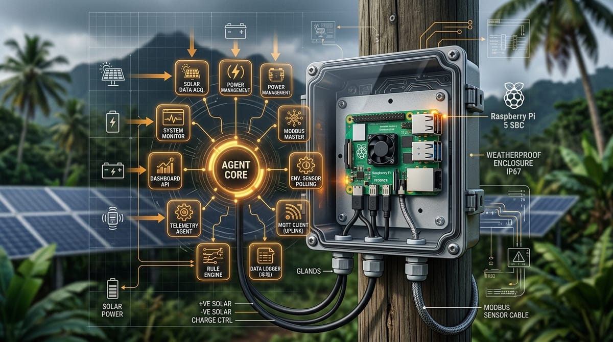
We set out to build a system that could change this. Not a dashboard in a data center, but an autonomous agent that lives at the microgrid — on an $80 single-board computer powered by the solar panels it manages. The result is microgrid-agent: an open-source Rust kernel that perceives, predicts, optimizes, and actuates a renewable energy microgrid with zero human intervention.
This is the fifth and final post in the Fleet Intelligence series. We have covered the problem (Colombia's energy paradox), the architecture (why agents, not SCADA), the forecasting stack, and the domain adaptation strategy. Now we ship it.
Why Rust
The choice of language was not academic. The agent runs on a Raspberry Pi 5 with 8 GB of RAM, deployed in tropical conditions with unreliable power. Every engineering decision flows from three constraints:
No garbage collection pauses. The control loop reads sensors at 1 Hz and dispatches power every 5 seconds. A 200 ms GC pause from Python or Java can mean a missed Modbus read cycle. Rust gives us deterministic latency — every allocation is known at compile time.
Single static binary. The compiled kernel is approximately 15 MB and cross-compiles from an x86 development machine to ARM64 with cargo build --target aarch64-unknown-linux-gnu. No runtime dependencies, no virtualenv, no JVM. Copy one file to the Pi, set up a systemd service, done.
Memory safety without runtime cost. The agent manages hardware interfaces — RS-485 serial, UART, GPIO. A memory corruption bug in a device driver does not just crash the process; it can send erroneous commands to a diesel generator or battery inverter. Rust's borrow checker catches these at compile time. The alternative is writing C and hoping the unit tests are thorough enough.
Cross-compilation is particularly important for fleet deployment. We build on CI, produce a single artifact per architecture, and distribute it over MQTT to every node in the fleet. No package manager resolution on a device with intermittent connectivity.
The Ten-Module Kernel
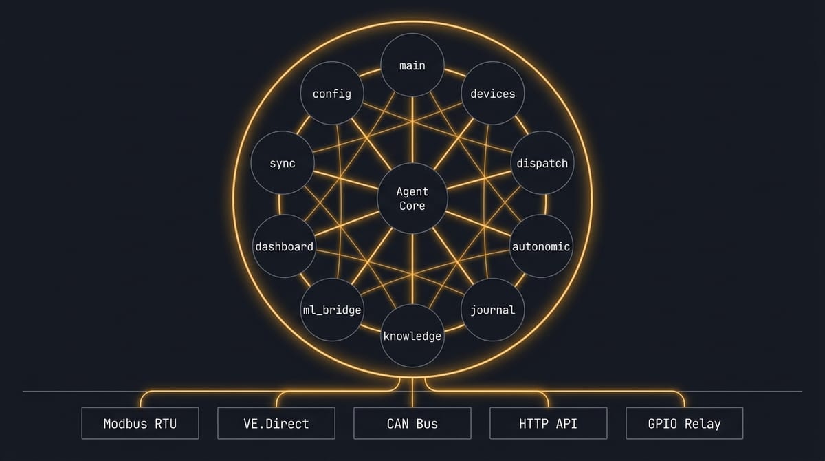
The agent binary consists of ten Rust modules, each with a single responsibility. Here is main.rs — the entire initialization sequence:
mod autonomic;
mod config;
mod dashboard;
mod devices;
mod dispatch;
mod journal;
mod knowledge;
mod ml_bridge;
mod sync;
mod tools;
The main function loads a TOML configuration file, initializes each subsystem, notifies systemd that the process is ready, and enters the control loop:
let agent = Agent {
    config,
    journal,
    knowledge,
    autonomic,
    devices,
    dispatcher,
    ml,
    fleet_sync,
    shadow: cli.shadow,
};
The control loop uses tokio::select! to multiplex four concurrent timers — sensor reads (1 Hz), dispatch optimization (every 5 seconds), ML forecasting (every 15 minutes), and a systemd watchdog heartbeat (every 20 seconds):
loop {
    tokio::select! {
        _ = sensor_interval.tick() => {
            // PERCEIVE: read all sensors
            if let Ok(readings) = self.devices.read_all().await {
                state.update_readings(readings);
                self.journal.append_readings(&state.latest_readings)?;
            }
        }
        _ = dispatch_interval.tick() => {
            // OPTIMIZE: compute dispatch
            let decision = self.dispatcher.solve(&state, &self.knowledge).await;
            // SAFETY: autonomic check — may override
            let final_decision = self.autonomic.enforce(decision, &state);
            // ACTUATE: send commands (unless shadow mode)
            if !self.shadow {
                self.devices.actuate(&final_decision).await?;
            }
            self.journal.append_decision(&final_decision)?;
        }
        _ = forecast_interval.tick() => {
            // PREDICT: spawn Python ML worker
            match self.ml.request_forecast(&state.history).await {
                Ok(forecast) => state.forecast = Some(forecast),
                Err(e) => {
                    state.forecast = Some(self.ml.persistence_fallback(&state.history));
                }
            }
        }
        _ = watchdog_interval.tick() => {
            let _ = sd_notify::notify(false, &[sd_notify::NotifyState::Watchdog]);
        }
    }
}
Each tick of the loop follows the PERCEIVE-PREDICT-OPTIMIZE-ACTUATE cycle from IEEE 2030.7, the standard specification for microgrid controllers. Shadow mode lets us deploy the agent alongside an existing system, logging what it would do without touching hardware — essential for validation.
Hardware Abstraction: Five Protocol Adapters
Every microgrid component speaks one of roughly four protocols. The agent does not need to know whether it is reading a Victron or SMA inverter — it needs a protocol adapter. The EnergyDevice trait captures this:
trait EnergyDevice {
    fn read_power_kw(&self) -> f64;
    fn read_energy_kwh(&self) -> f64;
    fn read_status(&self) -> DeviceStatus;
    fn set_power_limit(&self, kw: f64) -> Result;
    fn start(&self) -> Result;
    fn stop(&self) -> Result;
}
Five implementations cover the equipment found in Colombian microgrids:
- ModbusRtuDevice — RS-485, the universal language of inverters and gensets. The agent reads SunSpec-compliant registers at specific addresses (40071 for AC power, 40354 for battery SOC) with ~150 ms round-trip per command.
- VeDirectDevice — Victron's UART protocol, common in small ZNI installations. A simple text stream (
PPV\t320\r\n) parsed at 1 Hz over/dev/ttyUSB0. Important note: Victron uses 5V logic; the Pi's GPIO is 3.3V, requiring either a logic level converter or the galvanically isolated VE.Direct-to-USB cable ($35). - CanBusDevice — Some industrial controllers speak CAN bus (ISO 11898), common in genset ECUs from DSE and ComAp.
- HttpApiDevice — Modern smart inverters expose REST APIs over the local network.
- GpioRelayDevice — Simple on/off for basic gensets that lack any digital interface. Sometimes the most reliable option.
The DeviceRegistry wraps all of these behind a single read_all() and actuate() interface. In simulation mode (the --simulate flag), the registry substitutes a SimulatedDevice that produces a sinusoidal solar curve and random load — sufficient for all 155 tests to pass without any hardware attached.
The Autonomic Safety Layer
This is the part that keeps me sleeping at night. The AutonomicController is the last gate before any command reaches hardware. It enforces five hard constraints that no optimizer, no ML model, and no future LLM reasoning core can override:
// Shield 1: Never discharge battery below minimum SOC
if soc <= self.min_soc_pct && decision.battery_kw < 0.0 {
    warn!("OVERRIDE: Blocking battery discharge — SOC at minimum");
    decision.battery_kw = 0.0;
    was_overridden = true;
}

// Shield 2: Never overcharge battery
if soc >= self.max_soc_pct && decision.battery_kw > 0.0 {
    warn!("OVERRIDE: Blocking battery charge — SOC at maximum");
    decision.battery_kw = 0.0;
    was_overridden = true;
}

// Shield 3: Auto-start diesel when SOC critically low
if soc <= self.diesel_start_soc_pct && !decision.diesel_start {
    warn!("OVERRIDE: Auto-starting diesel — SOC critically low");
    decision.diesel_start = true;
    decision.diesel_kw = 5.0;
    was_overridden = true;
}

// Shield 4: Auto-stop diesel when SOC recovered
// Shield 5: Daily diesel runtime limit
Every override is logged with the word OVERRIDE in the tracing output. Every decision — whether overridden or not — is persisted to the crash-safe journal. The autonomic layer follows the Life Agent OS pattern: observe the current state, compare against hard constraints, act with the minimum intervention necessary.
The constraints are configured per site in TOML, with sane defaults (minimum SOC 20%, maximum 95%, diesel auto-start at 25%, auto-stop at 60%, daily diesel limit of 16 hours). A community operator can adjust these with a text editor; they never need to touch code.
Crash-Safe Journal
Every sensor reading and every dispatch decision is written to an append-only event journal backed by redb — an embedded key-value store purpose-built for crash safety. The journal uses monotonic sequence numbers and transactional writes:
pub fn append_readings(&self, readings: &SensorReadings) -> anyhow::Result<()> {
    let payload = serde_json::to_vec(readings)?;
    let seq = self.next_seq("readings_seq")?;
    let write_txn = self.db.begin_write()?;
    {
        let mut table = write_txn.open_table(READINGS_TABLE)?;
        table.insert(seq, payload.as_slice())?;
    }
    write_txn.commit()?;
    Ok(())
}
If the power cuts out mid-write, the transaction rolls back. When the Pi reboots, the journal is intact up to the last committed event. We tested this explicitly — write five entries, drop the database handle (simulating a crash), reopen, verify all five are still there. This matters because ZNI sites lose power routinely.
The journal serves triple duty: local audit trail, training data for the ML models, and the source for fleet synchronization. When the MQTT connection comes back online, queued events are replayed to the central broker.
Knowledge Graph
The KnowledgeGraph module stores the site topology in SQLite — entities (loads, feeders, buildings, services), their relationships (feeds, contains, depends_on), and priority levels (0=normal, 1=essential, 2=critical). A recursive CTE query answers questions like "what loads are affected if feeder-2 trips?" in under a millisecond:
WITH RECURSIVE affected(id, depth) AS (
    SELECT ?, 0
    UNION
    SELECT e.target_id, a.depth + 1
    FROM affected a
    JOIN edges e ON e.source_id = a.id
    WHERE e.relation IN ('feeds', 'contains', 'depends_on')
      AND a.depth < 10
)
SELECT DISTINCT id FROM affected WHERE depth > 0
The health post gets priority 2 (critical). The water pump gets priority 1 (essential). Street lights get priority 0 (normal). When load shedding is required, the dispatcher consults the knowledge graph to shed non-essential loads first. This is not a feature request — it is how communities already think about their energy. The knowledge graph encodes their priorities into the optimization.
Fleet Sync: MQTT with Store-and-Forward
The FleetSync module publishes telemetry to a central MQTT broker. MQTT was originally designed in 1999 for monitoring oil pipelines over satellite links — exactly our connectivity profile. When cellular connectivity drops (common in Guainia and Choco), messages are written to a disk queue as timestamped JSON files:
fn queue_to_disk(&self, topic: &str, payload: &[u8]) -> anyhow::Result<()> {
    let timestamp = chrono::Utc::now().timestamp_nanos_opt().unwrap_or(0);
    let filename = format!("{}-{}.json", topic, timestamp);
    let path = self.queue_dir.join(filename);
    std::fs::write(&path, payload)?;
    Ok(())
}
When connectivity is restored, the queue is replayed in chronological order. Persistent MQTT sessions with QoS 1 (at-least-once delivery) ensure no telemetry is lost. For ultra-constrained satellite links (Swarm M138: 750 bytes per packet, $5/month), we plan to use MQTT-SN with 2-byte topic IDs to cut per-message overhead from ~100 bytes to ~10 bytes.
The fleet coordinator subscribes to topics organized by region and site:
fleet/{region}/status        # Node heartbeats
fleet/{region}/telemetry     # Data summaries
fleet/{region}/models/update # New model weights
site/{site_id}/dispatch      # Dispatch results
site/{site_id}/alerts        # Critical alerts
This same topic hierarchy works for 10 nodes or 1,664 nodes. The MQTT broker handles fan-out.
The $650 BOM
The complete bill of materials for a single agent node:
| Component | Cost (USD) |
|---|---|
| Raspberry Pi 5, 8 GB | $80 |
| 256 GB NVMe SSD (M.2 HAT) | $30 |
| 27W USB-C power supply | $12 |
| PiJuice battery UPS HAT | $50 |
| IP65 DIN-rail enclosure | $25 |
| Waveshare RS-485/CAN HAT | $15 |
| 4x SCT-013-030 current transformers | $20 |
| ADS1115 16-bit ADC | $5 |
| Irradiance sensor | $30 |
| BME280 temperature/humidity | $5 |
| Victron SmartShunt (SOC) | $100 |
| Quectel EC25 4G LTE modem | $30 |
| Swarm M138 satellite (fallback) | $120 |
| Cabling, terminals, fuses | $50 |
| Total | ~$572-850 |
Plus approximately $10/month for cellular and satellite connectivity. For context, a single technician visit to a remote ZNI costs $500-2,000 in boat fuel, accommodation, and labor. The entire agent node costs less than two visits.
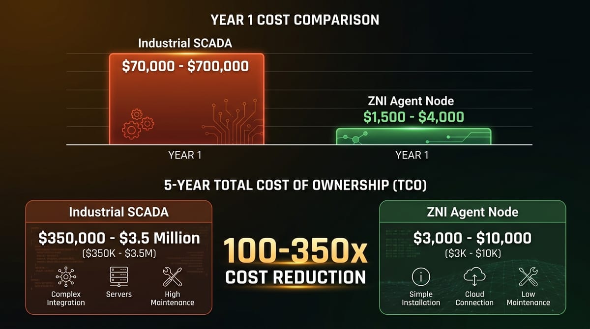
The Cost Gap: 100-350x Reduction
The research that grounds this project includes a detailed comparison with industrial microgrid management systems:
| Cost Component | Industrial | ZNI Agent Node | Ratio |
|---|---|---|---|
| Hardware | $5K-50K | $525-850 | 6-60x |
| Software license | $50K-500K/yr | $0 (open source) | -- |
| Installation | $10K-100K | $500-2K | 10-50x |
| Connectivity | $50-200/mo | $10-15/mo | 5-15x |
| Maintenance | $5K-50K/yr | $100-500/yr | 10-100x |
| Year 1 total | $70K-700K | $1.5K-4K | 17-175x |
| 5-year TCO | $350K-3.5M | $3K-10K | 100-350x |
The mathematical dispatch optimization is identical in both cases — the same LP/MILP formulation, the same HiGHS solver, the same constraints. Only the parameter values change. An LP that takes under a second on a Raspberry Pi for a 5-10 DER system with a 48-hour horizon at 15-minute timesteps is more than adequate.
At fleet scale, 100 agent nodes cost $87,000 in Year 1 — less than a single industrial SCADA deployment. And those 100 nodes generate collective intelligence: transfer learning between similar climate zones, fleet-wide anomaly detection, and a growing corpus of operational data that improves every forecast model.
155 Tests Passing
The prototype validates the architecture. Every module has unit tests, and the integration tests run entirely in simulation mode — no hardware required. This is intentional: any developer can clone the repo, run cargo test, and have a passing suite in under a minute.
Key test coverage includes:
- Autonomic shields: Verify that discharge is blocked at minimum SOC, charging is blocked at maximum, diesel auto-starts on critically low SOC, and the daily diesel runtime limit is enforced.
- Dispatch optimizer: Solar covers load before battery, battery discharges before diesel, excess solar charges battery, load shedding occurs only when all sources are exhausted.
- Journal crash safety: Write entries, drop the handle, reopen, verify all entries survived.
- Knowledge graph traversal: Linear chains, branching topologies, cycle detection (depth-limited CTE prevents infinite recursion), and priority load queries.
- Sensor simulation: Solar curve bounded by capacity, irradiance non-negative, SOC clamped to 0-100% after extreme charge/discharge.
- Fleet sync: Messages queue to disk with correct filename format, content survives round-trip.
The full test suite runs in CI on every push. Shadow mode deployment — where the agent reads real sensors but does not actuate — is the next validation step. The architecture separates perception from actuation precisely to enable this kind of incremental trust-building.
What's Next
This series has traced a path from Colombia's structural energy paradox through the architecture of autonomous fleet intelligence to a working prototype running on commodity hardware. The key ideas:
- Colombia's Energy Paradox — 1.9 million people with less than 6 hours of diesel power per day, while industry pays 39% above world average.
- Fleet Intelligence: Why Microgrids Need Autonomous Agents — SCADA monitors; agents decide. The control hierarchy collapses ISA-95 Levels 0-2 into a single edge node.
- The Three-Tier Forecasting Stack — PatchTST for hourly generation, foundation models for long-horizon demand, and why LLMs cannot predict power output.
- From Refinery to Selva — Domain adaptation transfers industrial operational knowledge to data-scarce ZNI sites.
- Edge Agents in the Wild (this post) — The Rust kernel, the hardware interface, the safety layer, and the $650 BOM.
The microgrid-agent repository is open source at github.com/broomva/microgrid-agent. The next milestones are shadow-mode deployment at a pilot site, integration with real Modbus and VE.Direct hardware, and federated model training across the first multi-node fleet. The math is identical at every scale. The architecture is ready. What remains is the patient work of earning trust — one autonomous decision at a time, with every decision logged, every override explained, and every watt accounted for.