The Three-Tier Forecasting Stack
Every autonomous microgrid agent needs to answer a deceptively simple question: how much solar power will this panel array produce in the next four hours? Get it right and you charge batteries at the optimal time, avoid diesel, and keep the lights on. Get it wrong and a community in Guainia loses electricity at 7 PM, or an industrial facility burns $4,000 in unnecessary diesel fuel overnight.
The forecasting problem for edge-deployed microgrids is unlike the one that leaderboard chasers work on. You are not predicting Walmart sales with five years of clean data. You are predicting solar irradiance in a location that may have zero historical operational data, on a device with 8 GB of RAM and no GPU, running on the same battery you are trying to optimize. The constraints are non-negotiable:
| Constraint | Value |
|---|---|
| Hardware | Raspberry Pi 5, ARM64, 8 GB RAM, no GPU |
| Inference budget | < 5 ms per forecast cycle |
| Model size | < 10 MB on disk |
| Cold-start | Must produce usable forecasts at new sites with zero local data |
| Connectivity | Intermittent — must work offline for days or weeks |
| Power | Runs on solar-charged battery; inference must be energy-efficient |
This post is about the architecture we chose to meet those constraints, the benchmarks that drove the decision, and the critical finding that LLMs — despite generating impressive demos — are fundamentally the wrong tool for numerical time-series prediction.
The Evolution: From ARIMA to Transformers to Foundation Models
The history of energy forecasting follows a predictable arc of increasing model complexity, and then — in an unexpected twist — a return to simplicity at the edge.
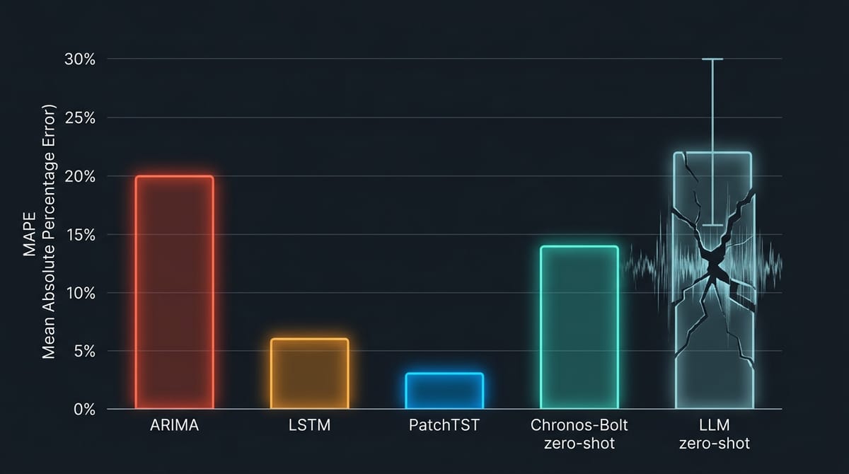
ARIMA and statistical methods (pre-2015) dominated for decades. They work well on stationary, univariate series with clear seasonality. Solar irradiance is none of those things — it is non-stationary, multivariate (temperature, humidity, cloud cover), and subject to abrupt regime changes (passing clouds, dust storms, panel degradation). ARIMA models typically achieve MAPE of 15-25% on solar, which is not good enough to dispatch batteries effectively.
LSTMs and recurrent networks (2015-2022) were the breakthrough. A 2-layer LSTM with 64 units achieves MAPE of 3-8% on solar forecasting given one or more years of site-specific training data. CNN-LSTM hybrids push this down to 2.5-5%. These models are tiny (~100K parameters, ~800 KB quantized to INT8), run in under 0.5 ms on a Raspberry Pi 5, and have been the workhorse of production energy forecasting for nearly a decade.
But LSTMs have a fatal limitation for our use case: they cannot zero-shot. An LSTM trained on an industrial solar farm in La Guajira knows nothing about a community microgrid in Choco. Transfer learning helps — MAPE degrades by only ~4 percentage points when transferred across sites — but you still need 3-12 months of data to train from scratch, and 2-4 weeks of target data to fine-tune a transferred model. When you are deploying to 1,664 ZNI localities, most of which have never had any instrumentation, "collect data for three months before the system works" is not an acceptable answer.
Transformer architectures (2022-present) changed the game. PatchTST, introduced at ICLR 2023, proved that attention mechanisms could outperform LSTMs on long-horizon forecasting — and do it with better transfer learning characteristics. The key innovation: instead of feeding individual time steps into the transformer, PatchTST segments the time series into patches of 64 consecutive values and treats each patch as a token. This is the same intuition behind Vision Transformers (ViT) — local patterns within a patch are captured by the embedding, and attention operates over the relationships between patches.
Foundation models (2024-2026) took this further. Models like Chronos-Bolt (Amazon), TimesFM (Google), and Moirai-2 (Salesforce) are pre-trained on billions of time-series data points and can forecast any new series zero-shot — no fine-tuning required. The SPIRIT benchmark (2025) showed that foundation models outperform traditional state-of-the-art by approximately 70% on zero-shot solar irradiance prediction.
And then came the hype cycle's most dangerous idea: why not just use an LLM?
Why LLMs Cannot Predict Power
In late 2023, Gruver et al. published "Large Language Models Are Zero-Shot Time Series Forecasters" at NeurIPS. The paper demonstrated that GPT-3 and LLaMA-2, when given time series as digit strings, could produce forecasts comparable to purpose-built models on some benchmarks. The AI community responded with predictable enthusiasm. If LLMs can reason and forecast, why build specialized models at all?
The answer came 18 months later, and it was devastating.
Park et al. (ACL 2025) published "Revisiting LLMs as Zero-Shot Time-Series Forecasters: Small Noise Can Break Large Models." Their finding: LLM forecasters are extremely fragile to noise. Small perturbations in the input — the kind that are present in every real-world sensor reading — cause disproportionately large prediction errors. Worse: simple single-shot linear models (DLinear-S, RLinear-S), trained on only the input sequence itself, outperform LLM forecasters at a fraction of the inference cost.
This result is not surprising once you understand what LLMs actually do with numbers. LLMs tokenize digits as text. The number 1847.3 might be tokenized as ["18", "47", ".", "3"] — four tokens with no inherent numerical relationship. The model learns statistical co-occurrence patterns between digit strings, not the mathematical relationships between values. When the input is clean and periodic, these patterns happen to produce reasonable extrapolations. When the input is noisy — which solar irradiance data always is — the patterns break down.
The performance gap is not subtle:
| Approach | Same-Site MAPE | Transferred MAPE | Zero-Shot MAPE | Noise Sensitivity |
|---|---|---|---|---|
| LSTM (2-layer, 64 units) | 3-8% | 8-15% | N/A | Low |
| PatchTST | 2-5% | 5-10% | N/A | Low |
| Chronos-Bolt (zero-shot) | -- | -- | 10-18% | Moderate |
| TimesFM 2.5 (zero-shot) | -- | -- | 10-18% | Moderate |
| LLM zero-shot (Gruver et al.) | -- | -- | 15-30% | Extreme |
| Hybrid (PatchTST + physics + TSFM bootstrap) | 2-5% | 4-8% | 8-15% | Low |
But the numbers only tell half the story. The resource cost tells the rest.
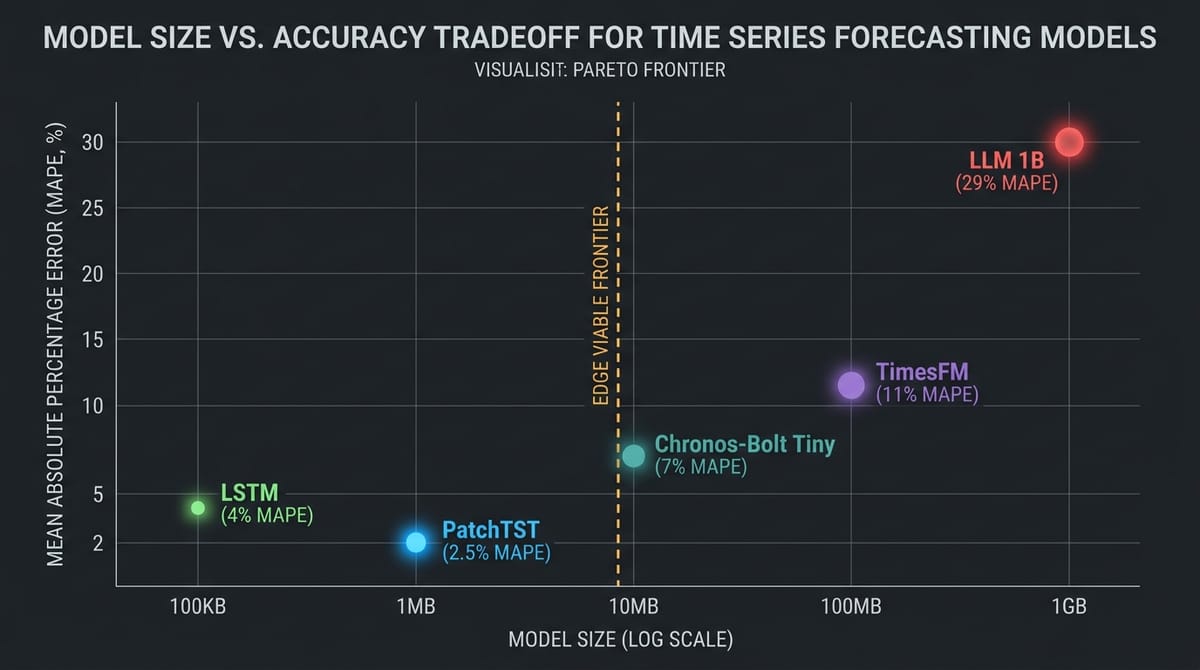
A quantized PatchTST model on a Raspberry Pi 5 produces a 24-hour, 15-minute-resolution forecast (96 time steps) in under 2 milliseconds. It occupies 1-5 MB of disk and 100-200 MB of RAM.
A 1B-parameter LLM quantized to 4-bit on the same Raspberry Pi 5 produces the same forecast in approximately 25 seconds. It occupies 700 MB of disk and 2 GB of RAM — RAM that the agent needs for its knowledge graph, its optimization engine, its communication stack, and its operating system.
The LLM is 25,000x slower for an equivalent or worse result. On a device powered by the same solar panel it is trying to forecast, those 25 seconds of compute are not just slow — they are an energy cost that directly reduces the battery capacity available for the community.
| Model | Parameters | Disk (INT8) | RAM | Inference (RPi 5) | Edge Viable? |
|---|---|---|---|---|---|
| LSTM (2-layer, 64u) | ~100K | ~800 KB | ~20 MB | < 0.5 ms | Yes |
| Lightweight PatchTST | ~50-500K | ~250 KB | ~50-100 MB | < 1 ms | Yes |
| PatchTST | ~1-5M | ~1-5 MB | ~100-200 MB | < 2 ms | Yes |
| Chronos-Bolt Tiny (9M) | 9M | ~9 MB | ~200-500 MB | ~100-500 ms | Yes (bootstrap only) |
| Chronos-Bolt Mini (21M) | 21M | ~21 MB | ~500 MB-1 GB | ~0.5-2 s | Marginal |
| TimesFM 2.5 (200M) | 200M | ~200 MB | ~2-4 GB | ~5-15 s | No |
| LLM 1B (Q4) | 1B | ~700 MB | ~2 GB | ~25 s (96 steps) | No (as forecaster) |
This does not mean LLMs have no role in microgrid management. It means their role is not prediction. More on that in a moment.
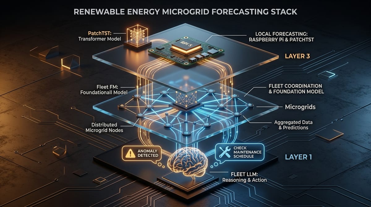
Tier 1: PatchTST at the Edge
PatchTST is the primary forecaster on every edge node in the fleet. Here is why.
The core insight of PatchTST (Nie et al., ICLR 2023) is that a time series is worth 64 words. Instead of treating each time step as a separate token — which creates quadratic attention complexity over hundreds of steps — PatchTST groups consecutive time steps into non-overlapping patches of length 64 and embeds each patch as a single token. A 24-hour lookback at 15-minute resolution (96 time steps) becomes just 2 tokens (with padding). A one-week lookback becomes 10-11 tokens.
This has three consequences for edge deployment:
-
Dramatically reduced attention cost. Attention is O(n^2) in the number of tokens. With 10 tokens instead of 672, the computational cost drops by roughly 4,500x.
-
Local pattern preservation. Each patch embedding captures the local temporal structure (daily cycles, ramp patterns, cloud transients) as a single learned representation. These local patterns transfer well between sites because the physics of solar irradiance creates similar local dynamics everywhere.
-
Channel independence. PatchTST processes each variable (solar output, demand, battery SOC, temperature) as an independent channel with shared patch embeddings. This means the model naturally handles multivariate microgrid data without cross-variable attention overhead.
Quantized to INT8, a PatchTST model with 1-5M parameters occupies 1-5 MB on disk and runs in under 2 ms on a Raspberry Pi 5. A recent KDD MiLeTS 2025 workshop paper showed that PatchTST can be quantized to 4-bit with competitive accuracy — at which point a 500K-parameter model is approximately 250 KB. That is smaller than an INT8 LSTM.
For transfer learning, the architecture offers a clean fine-tuning protocol: freeze the patch embedding layer (which captures domain-invariant local patterns) and fine-tune only the attention heads and prediction head on the target site's data. With as little as 1-2 weeks of local data, a transferred PatchTST achieves MAPE of 5-10% — competitive with an LSTM trained on 3-12 months of data.
The LSTM is not discarded. It remains as a battle-tested fallback with known TFLite behavior, deployed alongside PatchTST on every node. If the PatchTST model encounters convergence issues or an edge case that destabilizes its predictions, the system falls back to the LSTM automatically based on a rolling accuracy comparison.
Both models are wrapped with a conformal prediction layer that produces calibrated uncertainty intervals without distributional assumptions. The dispatch optimizer does not receive a point forecast — it receives a forecast with a confidence band. When the band is wide, the optimizer makes conservative decisions (keep diesel on standby, reduce battery discharge depth). When the band is narrow, it can be aggressive (delay diesel start, maximize battery throughput). This is how uncertainty becomes operationally useful rather than merely statistical.
Tier 2: Fleet Intelligence with Foundation Models
A PatchTST that has never seen any data from a site cannot forecast anything. The cold-start problem is the fundamental challenge of deploying to 1,664 ZNI localities — most of which have never been instrumented.
This is where foundation models enter the architecture, not as the primary forecaster but as the bootstrap layer.
Chronos-Bolt Tiny (Amazon, 9M parameters) is designed for CPU deployment. At approximately 9 MB quantized to INT8 and requiring 200-500 MB of RAM, it can run on a Raspberry Pi 5 as a bootstrap-only model. When a new node is deployed with zero local data, Chronos-Bolt provides zero-shot forecasts that, according to the SPIRIT benchmark, outperform previous state-of-the-art by ~70% in the zero-shot regime.
The 2026 Energy Load Forecasting Benchmark (arXiv:2602.10848) evaluated Chronos-Bolt, Chronos-2, and Moirai-2 across 2,300+ forecast scenarios on consumer hardware. A critical finding: as context length increased from 24 to 2,048 hours, Chronos-Bolt improved by 43% and Moirai-2 improved by 76%. More context means dramatically better forecasts — but longer context means more memory and compute. The tiny variant strikes the right balance for edge bootstrap.
At the fleet coordinator level — a server-class machine (or cloud instance when connectivity is available) — larger foundation models like Chronos-Bolt Small (48M) or TimesFM 2.5 (200M) provide higher-quality zero-shot predictions and generate pre-training weights that are distilled into edge-deployable PatchTST models.
The fleet coordinator also runs federated learning via the Flower framework. Each Raspberry Pi acts as a federated learning client; the coordinator is the server. Model weight updates (~200 KB per round after quantization) are synced via MQTT when connectivity is available. Critically, the aggregation is climate-clustered: nodes in the Colombian Pacific (3.0-3.5 kWh/m^2/day solar irradiance, extreme cloud cover) share updates only with other Pacific nodes. Orinoquian sites (4.5-5.5 kWh/m^2/day, seasonal flooding) share with their climate peers. This prevents negative transfer — a model trained on La Guajira's consistent 6.0+ kWh/m^2/day irradiance would hurt, not help, a Pacific site.
The lifecycle of a node's forecasting capability follows a clear progression:
- Day 0: Deploy with Chronos-Bolt Tiny zero-shot. MAPE ~10-18%. Usable but not optimal.
- Weeks 1-2: Collect local data. Begin fine-tuning PatchTST from fleet-provided pre-trained weights.
- Month 1: PatchTST takes over as primary forecaster. MAPE ~5-10%. Chronos-Bolt enters standby.
- Ongoing: Federated learning continues to improve the model. Climate-clustered peers share their patterns. MAPE converges toward 2-5% as the fleet grows.
Tier 3: The LLM Reasons About Forecasts
The third tier is where the LLM lives — and its job description is explicitly not prediction.
The agent's Arcan runtime consumes PatchTST forecasts as input to its decision engine. When the forecast says solar output will drop 40% tomorrow, the LLM's role is to reason about why and what to do about it:
- "Solar forecast dropped 40% — the knowledge graph shows a seasonal cloud pattern for this week in Choco. This is expected. Pre-charge batteries to 90% today."
- "Demand spike predicted at 7 PM — the knowledge graph shows a community event was registered. Shift non-critical loads to 5 PM."
- "Panel efficiency has declined 12% over six weeks — schedule cleaning during next technician visit."
- "Forecast confidence interval is abnormally wide — possible sensor degradation. Flag for remote diagnostic."
This is what LLMs are genuinely good at: causal reasoning, knowledge graph traversal, natural language summarization, and connecting disparate pieces of context. They are terrible at producing the number 1847.3 from a noisy sequence of prior numbers. They are excellent at explaining why that number matters and what to do about it.
Implementation offers three fallback modes depending on connectivity:
- Connected: Cloud LLM API for full reasoning capability
- Offline (8 GB RPi): A 1B quantized model (Q4, ~2 GB RAM) for basic reasoning
- Degraded: Rule-based heuristics that cover the most common operational decisions without any language model
The key design principle: the system never depends on the LLM being available to operate safely. Dispatch decisions can be made purely from PatchTST forecasts and optimization constraints. The LLM makes the system smarter, not functional.
The Physics Layer That Makes Transfer Learning Work
One technique deserves its own section because it has an outsized impact: clear-sky normalization.
Nie et al. (2024) demonstrated that normalizing solar output by the theoretical clear-sky irradiance for a given location and time transforms the forecasting target from "absolute power" (highly domain-specific — depends on latitude, panel tilt, equipment specs) to "clear-sky index" (domain-invariant — captures the cloud and atmospheric effects relative to the physical maximum).
Clear-sky irradiance curves are available for free from the European Commission's PVGIS API for any coordinate on Earth. You precompute the curve for each ZNI site, store it in the knowledge graph, and divide measured power by clear-sky irradiance at each time step. The model now predicts how much of the theoretical maximum will be achieved — a value between 0 and 1 that transfers far better between sites than raw wattage.
This single normalization step makes zero-shot and few-shot results competitive with months of site-specific training. Combined with PatchTST's patch embeddings (which already capture transferable local patterns) and physics-informed loss constraints (solar output cannot exceed rated capacity, must be zero at night, follows known temperature-power coefficients), the system bootstraps effectively from physics before it has any operational data at all.
The Resource Budget
On a Raspberry Pi 5 with 8 GB of RAM, the complete forecasting stack fits comfortably:
| Component | RAM | Disk | Inference Time |
|---|---|---|---|
| PatchTST forecaster (INT8) | 100-200 MB | 1-5 MB | < 2 ms |
| LSTM fallback (INT8) | 20 MB | 800 KB | < 0.5 ms |
| Conformal prediction wrapper | 10-20 MB | -- | < 1 ms |
| Chronos-Bolt Tiny (bootstrap) | 200-500 MB | 9 MB | ~100-500 ms |
| Forecasting total | ~330-740 MB | ~12 MB | < 5 ms (steady state) |
This leaves 4-5 GB for the Arcan agent runtime, the knowledge graph (SQLite), the event journal (redb), the dispatch optimizer, the local dashboard, and — optionally — a 1B quantized LLM for offline reasoning. The forecasting stack does not compete for resources because it was designed from the start to be a lightweight, high-frequency component that produces inputs for heavier reasoning processes.
What's Next
This is the third post in a five-part series on Fleet Intelligence for Renewable Microgrids:
- Colombia's Energy Paradox: 39% Above World Average and 1.9M People in the Dark
- Fleet Intelligence: Why Microgrids Need Autonomous Agents, Not Better SCADA
- The Three-Tier Forecasting Stack <-- you are here
- From Refinery to Selva: Domain Adaptation for Energy AI
- Edge Agents in the Wild: Rust, Raspberry Pi, and Autonomous Microgrids
The next post dives into the transfer learning problem: how do you take a model trained on an Ecopetrol industrial solar farm (6.0+ kWh/m^2/day, clean data, stable grid) and adapt it to a community microgrid in Coqui, Choco (3.0 kWh/m^2/day, no historical data, intermittent connectivity)? The answer involves federated learning, climate clustering, and a few counterintuitive findings about what transfers and what doesn't.
Code: github.com/broomva/microgrid-agent (155 tests passing, simulation framework included).
Based on a review of 30+ papers (2023-2026) including benchmarks from SPIRIT (2025), the Energy Load Forecasting Benchmark (2026), and the critical Park et al. ACL 2025 study on LLM forecasting fragility.